Feature Attribution in Computer Vision

Feature attribution methods help us understand how a particular neural network architecture makes it's prediction. The most common (and simple) feature attribution method is called a saliency map — a simple heatmap that highlights pixels of the input image that most likely caused the output. In today's workshop, we learn more about such maps and the different methods that can be used to obtain them.

Learning Objectives

• Understand how to use Vanilla Gradients for feature attribution
• Understand how to use Grad-CAMs for feature attribution

Saliency maps using vanilla gradients

Saliency maps based on vanilla gradients use backpropogation to provide us with insight on which areas of the image play key role in discrimating between classes.

Before we go deeper in Saliency maps, let's take a small detour to Block B: in particular linear models.

Recall that a linear model is written as:

y = β^T.X

Where,

β (beta) : vector of regression coefficients
X : matrix of predictor variables.
Y : vector of the outcome variable.

Replacing β (beta-regression terminology) with w (weights-neural network terminology), we have

y = w^T.X

Expanding the equations across n cases, we have

y = w₁x₁ + w₂x₂ + … + w_nx_n

In this equation, the gradients aka the weights answer the question - how much does a unit change in x affect y. e.g., A 1 unit change in x₁ would result in a w₁ units change in y. Thus by plotting the weights, we can quantify the relative contribution of each feature (the x's) to the final prediction!

Recall that neural networks use backpropogation to learn the weights of each connection, which are then used to make the final predictions. A gradient, in general terms measures the change in an output, when the inputs are perturbed. In the context of backpropogation, the gradients carry information about the relative importance of the weights in the neural network towards the final classification. In particular, the magnitude of the gradients quantifies the contribution of a particular connection in the neural network to the final classification probability. In backpropogation, we initialize the network with random weights, and use gradient descent to optimally adjust the weights such that we minimize the final cost function (or maxmimise the classification accuracy). Please watch this video to refresh your memory on backpropogation.

Saliency maps extend this idea to provide intuitive explanations of why a certain image is assigned a specific class. Let's start by considering an image classifier which has been trained on labelled images of cats and dogs and we have tuned the model such that we have excellent performance on the test set. However, what we would like to explore is - how is the model able to discrimate so accurately between a cat and a dog aka can we explain the model's predictions! We provide the learned neural network with the image of a cat, predict the label (=cat), and then do a single pass of backpropogation to obtain the gradients for that given image. We can use these gradients to highlight input regions that cause the most change in the output. Intuitively this should highlight salient image regions that most contribute towards the output!

Saliency maps using Grad-CAMs

Similar to vanilla gradients, Grad-CAM provides visual explanations for CNN decisions. Unlike other vanilla gradients, the gradient is not backpropagated all the way back to the image, but to the last convolutional layer to produce a map that highlights important regions of the image.

Let us start with an intuitive consideration of Grad-CAM. The goal of Grad-CAM is to understand at which parts of an image a convolutional layer "looks" for a certain classification. As a reminder, the first convolutional layer of a CNN takes as input the images and outputs feature maps that encode learned features (see the chapter on Learned Features). The higher-level convolutional layers do the same, but take as input the feature maps of the previous convolutional layers. To understand how the CNN makes decisions, Grad-CAM analyzes which regions are activated in the feature maps of the last convolutional layers.

Saliency maps using SmoothGrad

One of the key drawbacks of vanilla gradients and Grad-CAM is that they resulting saliency maps can sometimes be very noisy. One way of dealing with is to first create multiple versions of the image with varying levels of noise. Then we create saliency maps using Grad-CAM for all the images and later, average the saliency maps to produce a final (usually noise free) map. In essense, we are trying to average away the noise.

Let's get to work!

Today, we have discovered three new ways to explain how do neural networks make their decisions! Now let's put them to to the test and see how they perform using the tf_explain python package.

Click here to read more about the package.

Start by ensuring that you first install the tf_explain library. Feel free to do this in google colab, either on the cloud or your local runtime. I recommend using your local runtime as it will be easier when you want to apply it to your creative brief.

!pip install tf_explain
!pip install opencv-python

Next we load the required libraries. Note that tf_explain provides functions for the following saliency maps.

• Activations Visualization
• Vanilla Gradients
• Occlusion Sensitivity
• Grad CAM (Class Activation Maps)
• SmoothGrad
• Integrated Gradients

In this workshop, we focus on the highlighted method.

Now we can load the required libraries and functions. Let's start with GradCAM.

#load libraries
import numpy as np
import tensorflow as tf
import PIL

#load GradCAM
from tf_explain.core.grad_cam import GradCAM

For this example, we are going to use a pre-trained model , the VGG16 architecture which was trained on ImageNet. Lastly, we are going to use the internet's favourite image, a tabbycat to investigate saliency maps. Note that, in the image net dataset, a tabby cat is assigned a class label of 281, we will come back to this later.

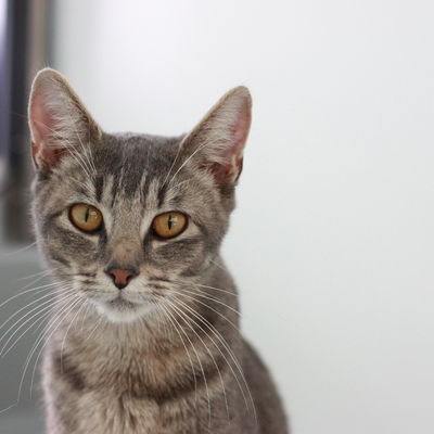
We being by first setting the image path and it's class label.

IMAGE_PATH = "C:/Users/bhushan.n/Desktop/cat.jpg"
class_index = 281

Note that this path will change for you, and also depend on whether you are using a local or hosted runtime.

Next, we can preprocess the image so it's ready for keras and VGG16. Note that the model expects the input image to be of size 224 X 224.

img = tf.keras.preprocessing.image.load_img(IMAGE_PATH, target_size=(224, 224))
img = tf.keras.preprocessing.image.img_to_array(img)

Now we load the pre-trained VGG16 model using the following line of code.

model = tf.keras.applications.vgg16.VGG16(weights="imagenet", include_top=True)
#get model summary
model.summary()

What does include_top=TRUE do, and also investigate what happends if we set it to FALSE

So now that we have loaded the image and loaded the model. We are ready to use tf_explain to understand what does VGG16 see when it classifies this image as a cat.

#first create the input in a format that the explainer expects (a tuple)
input_img = (np.array([img]), None)

#initialize the explainer
explainer = GradCAM()

# Compute GradCAM on VGG16
grid = explainer.explain(input_img,
                         model,
                         class_index=class_index
                         )

#save the resulting image
explainer.save(grid, "C:/Users/bhushan.n/Desktop/", "grad_cam.png")

And voila!

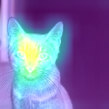
Let's place the images closer for comparison

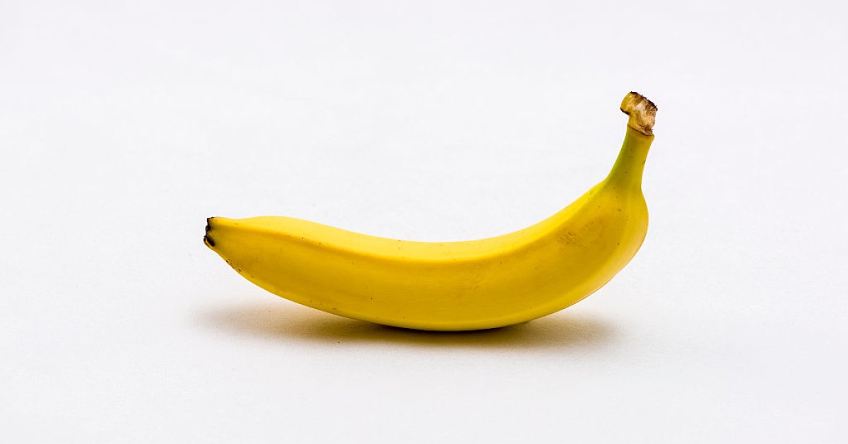
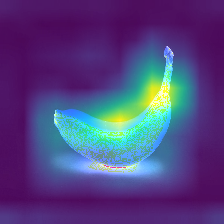
Here's another example, this time a banana.

Optional: A deeper understanding

To get a deeper understanding of how these methods work and their technical underpinnings, please watch the following lecture. If you find some concepts tricky to understand, take notes and bring them to class where we can discuss them.

Assignments

• {optional} Watch this video to understand more about the software package developed to implement these methods. Please keep in mind that this package is still in it's development stage (and bugs are to be expected).

• Use any image (no cats please) and a corresponding imagenet class to explore what do neural networks (in particular, VGG16) see when they classify that image. Specifically,
  • Go here for a mapping of class labels to human descriptions
  • Use any label you find interesting (e.g., Banana) note down the class label index
  • Use google search to search for images of the class you have chosen.
  • Load the image into your script (don't forget to change the class_index variable)
  • Starting with GradCAM, try several XAI methods and save your findings.
  • Compare the methods qualitatively in a table.
  • Upload your script, saliency maps, and qualitative comparisons to github.