Datalab 04: Perceptron

In today's DataLab session you are going to apply the perceptron algorithm to the youth care dataset.

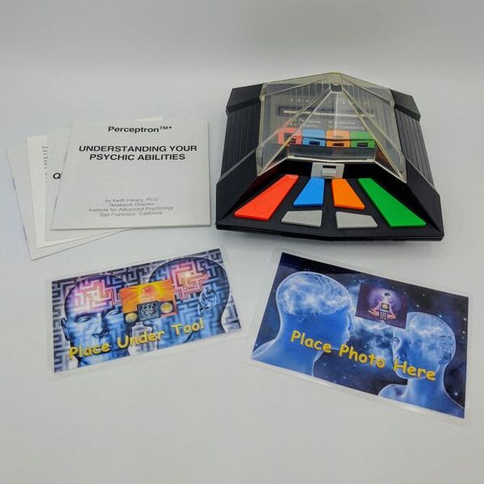
Figure 1. Another perceptron…

I found another example of a ‘perceptron' online. Apparently, this version helps you to discover, and explore your ‘psychic abilities', interesting to say the least .

Learning Objectives:

1. Apply appropriate pre-processing techniques to the youth care dataset
2. Train, and evaluate the perceptron on the youth care dataset

Table of contents:

1. Oosterhout Dataset: Perceptron: 4 hours
2. Additional material (optional): 3 hours 2.1 Perceptron: Activation functions 2.2 Feature scaling
3. In-Class discussion

Questions or issues?

If you have any questions or issues regarding the course material after the Q&A, please first ask your peers or ask us if you can't figure it out together!

Good luck!

0) Stand-up

We start by hosting a stand-up. Form groups of ~ 5 and run on-another through the following points:

• What progress have you made up since last datalab?
• What progress do you anticipate to make today?
• What impediments are you facing or expecting?
• With what could you use help or support?

Open your worklog and plan your day informed by the stand-up and today's schedule

1) Q & A

We start by briefly reflecting on what we learned about classification algoritms, overfitting and the bias-variance trade-off. Do you have any questions? Now is the time to ask them!

1) Oosterhout Dataset: Perceptron

Document your code

Write your argumentation down in a in-line comments; and for every line of code: write an in-line comment explaining what the line of code does exactly. Figure 1. below is a good demonstration of documented code.

The example script I provided in Data Science 1 is also a good example of how to document your code; albeit that one was done in R.

1. Open your python file (MachineLearning_OosterhoutModels_…) used for the final delivery of your model.
2. Load in the youthcare dataset you created in Business Intelligence if you haven't done so already. Load in any other data you might need. Then save your file to your GitHub repository.
3. Open your research design and use in-line comments to formulate a classification analysis using the perceptron algorithm based on your research question (or when not answerable using this type of analysis: perform an analysis related to your research question). Start by listing the variables which you think could predict the outcome variable you're interested in and motivate why you think they might predict your outcome variable.
4. Implement the perceptron algorithm. You can either choose to use the Python code from Codecademy, which implements the original perceptron by Rosenblatt or you can use the scikit-learn function (linear_model.Perceptron()), which implements a more modern version of the perceptron (see Additional material section!).
5. Test, re-fit and validate your model. Create a new model on a new line for every re-fit. Keep track of any predictor variables you exclude from the full model when re-fitting. Motivate why you are excluding; or including new variables using in-line comments.
6. Continue till 16:00, or stop when you feel you can no longer improve the model. Then save your file to your GitHub repository.

2) Additional material (optional)

The perceptron has many different implementations, also referred to as architectures. Today, we will focus on one element of the perceptron architecture, the threshold or activation function.

2.1 Perceptron: Activation functions

As you may have read, one of the main elements of the perceptron algorithm is the activation function. There are three types of activation functions: non-differentiable, subdifferentiable, and differentiable:

1. Non-differentiable (Gradient descent ):

• Heaviside, or unit step

The original perceptron developed by Rosenblatt uses this particular activation/threshold function. This variation of the perceptron only accepts binary (i.e. 0 or 1) input variables, and its activation function is non-differentiable. Meaning, gradient descent will not help to optimize the performance of the model because the gradients are almost always zero (except when x = 0).

Function	Plot	Equation	Derivative
Heaviside/Unit Step

Figure 2. Heaviside activation/threshold function.

Limitation of the Heaviside function, exemplified:

• A small change in the weights and/or biases in the network can cause the output of the perceptron to radically change from 0 to 1 (i.e. change category!) Solution: Differentiable or sub-differentiable activation function.

Learning algorithms sound terrific. But how can we devise such algorithms for a neural network? Suppose we have a network of perceptrons that we'd like to use to learn to solve some problem. For example, the inputs to the network might be the raw pixel data from a scanned, handwritten image of a digit. And we'd like the network to learn weights and biases so that the output from the network correctly classifies the digit. To see how learning might work, suppose we make a small change in some weight (or bias) in the network. What we'd like is for this small change in weight to cause only a small corresponding change in the output from the network. As we'll see in a moment, this property will make learning possible.
If it were true that a small change in a weight (or bias) causes only a small change in output, then we could use this fact to modify the weights and biases to get our network to behave more in the manner we want. For example, suppose the network was mistakenly classifying an image as an "8" when it should be a "9". We could figure out how to make a small change in the weights and biases so the network gets a little closer to classifying the image as a "9". And then we'd repeat this, changing the weights and biases over and over to produce better and better output. The network would be learning.
The problem is that this isn't what happens when our network contains perceptrons. In fact, a small change in the weights or bias of any single perceptron in the network can sometimes cause the output of that perceptron to completely flip, say from 0 to 1. That flip may then cause the behaviour of the rest of the network to completely change in some very complicated way. So while your "9" might now be classified correctly, the behaviour of the network on all the other images is likely to have completely changed in some hard-to-control way. That makes it difficult to see how to gradually modify the weights and biases so that the network gets closer to the desired behaviour. Perhaps there's some clever way of getting around this problem. But it's not immediately obvious how we can get a network of perceptrons to learn (Nielson, December 1, 2019).

2. Subdifferentiable (Gradient descent ):

• Rectified Linear Units (ReLU)

This is one of the most popular activation functions used in the field of deep learning. In this case, the gradient is only zero when x < 0. In other words, this algorithm can be optimized via gradient descent. This variation of the perceptron accepts both binary (i.e. 0 or 1) and continuous (i.e. between 0 and 1) input variables. As a result, it is a good practice to scale your continuous features.

Function	Plot	Equation	Derivative
Rectified Linear Units, ReLU

Figure 3. Rectified Linear Units activation function.

3. Differentiable (Gradient descent ):

• Sigmoid

Looks familiar? This is one of the most well-known activation functions. It is also used in logistic regression. The gradient is 0 when x = 0 or x = 1. This variation of the perceptron, also knows as the sigmoid neuron, accepts both binary (i.e. 0 or 1) and continuous (i.e. between 0 and 1) input variables. As a result, it is a good practice to scale your continuous features. The output of the model is continuous (i.e. between 0 and 1). In practice, the value 0.5 is frequently used as a decision-boundary: x ≤ 0.5 and x > 0.5.

Function	Plot	Equation	Derivative
Sigmoid

Figure 4. Sigmoid activation function.

Want to learn more about the sigmoid neuron, see the book chapter 1.3: Sigmoid neurons by Nielson (December 1, 2020).

Interested in exploring how gradient descent and backpropagation work, make sure to check the example by Mikael Laine:

Video 1. Neural Network Backpropagation Basics For Dummies by Mikael Laine.

2.2 Feature scaling

Feature scaling is a technique to standardize your predictors within a fixed range. scikit-learn defines it as follows:

Standardization involves rescaling the features such that they have the properties of a standard normal distribution with a mean of zero and a standard deviation of one (‘The Importance of', n.d.).

For an explanation of how feature scaling works, see scikit-learn's article Importance of Feature Scaling (n.d.).

Documentation (Python):

scikit-learn:

• StandardScaler()

3) In-Class discussion

At 16:00, there's a meeting you're encouraged to take part in to ask questions and to discuss our progress and reflect on today's activities.

#3 Up next! There's no new material to be covered, you should use the remainder of your time to work on your project brief and make the best model; and dashboard, you can possibly make!

Resources

• Codecademy